Monsters of the Movies - Achievement Unlocked

After almost forty years, I've finally managed to see all the films listed in Monsters of the Movies. I've been tracking my progress in a spreadsheet and a letterboxd list and over the last few months, I've been slowly filling my gaps by downloading the films from archive.org or watching the films online. The exception was Mad Love (1935), which I had to get through Amazon as a Spanish-subtitled DVD and then watch with the subtitles turned off!

Amongst the recently-watched films, the two stand-out gems for me were The Manster (1959) a.k.a. The Split:

and The Abominable Dr. Phibes (1971):

I kept the latter until the very end ... and I wasn't disappointed.

Lexicon 2

To finish off the discussion of my Lexicon demo, I'll outline the in-memory data structure used to store the dictionary.

In the first part, I described how the lexicon is stored trivially-compressed for transmission "over the wire". The words are then expanded in memory into a form that makes searching simple and efficient.

The main data structure is a four-dimensional array of JavaScript objects named "Lexicon.byRaritySubsetLength":

1. The first index is an integer rarity between one and five inclusive: one means "not very rare", whereas five means "esoteric".
2. The second index is an integer bit-field (one to seven inclusive) which encodes which dictionaries the corresponding list is part of: TWL06, SOWPODS and SCOWL.
3. The third index is the integer length of the word (two to fifteen inclusive).
4. The fourth index is an integer index into a list sorted alphabetically (starting from zero).

By default, the demo looks at all rarities and word lengths for the SOWPODS lexicon. This means that without changing the criteria, when matching words, the client must look through 5 * 4 * 14 = 70 lists of words.

Each word entry is a JavaScript object of the following form:

    word : string

    rarity : integer

    subset : integer

    mask : integer

The first three fields contain the uppercase word, rarity index and lexicon subset mask. The last field is used when searching for anagrams. It is a bit-field that encodes which letters are contained within the word: 1 for "A", 2 for "B", 4 for "C", 8 for "D", etc.

For instance, to find anagrams for "WORDS" in SOWPODS, the client needs to search through only 20 lists of words: five rarities (1 to 5), four lists for SOWPODS and one word length (5). These lists contain 12,478 entries which can be scanned quickly by looking for those that have a "mask" with the bits for "D", "O", "R", "S" and "W" all set. It will typically come up with the solution ("SWORD" and "DROWS") within a couple of milliseconds.

Mario T-Shirt

From an original idea by David Gavilan Ruiz

Mortality Statistics

The Office for National Statistics collects mortality data for the United Kingdom. There's lots of information hidden within the data, but some of it is quite difficult to extract and/or visualise.

The underlying data for questions of life expectancy and mortality rates would seem to be a statistic named "Qx" (raw data). According to their guide, this is defined by the ONS as:

The mortality rate between age x and (x +1); that is, the probability that a person aged x exactly will die before reaching age (x +1).

It is sometimes expressed as a probability multiplied by 100,000. You can plot this for males as a surface with one axis being the age, "x", and the other being the year of observation of "Qx":

The noise towards the "back" of the graph is due to the fact that concrete data beyond the age of 100 is very sparse, so probabilities are difficult to calculate accurately. The next derived value is "Lx" which the ONS defines as:

The number of survivors to exact age x of 100,000 live births of the same sex who are assumed to be subject throughout their lives to the mortality rates experienced in the 3-year period to which the national life table relates.

I've approximated that as a normalised probability:

L[0] = 1

L[i] = L[i-1] * (1 - Q[i-1])

This gives a monotonically decreasing graph that reminds me a bit of a zero curve from fixed-income finance.

You can already see that the shape of the "Lx" curve has changed appreciably between 1850 and 2000. But the graphs (which I prepared using the excellent plotly) become easier to interpret if we add more colour levels:

You can start to see that there are strange "striations" in the surface. We now look at "Dx", defined as:

The number dying between exact age x and (x +1) described similarly to Lx.

I used the following formula:

D[i] = L[i] - L[i+1]

This gives a surface that has a few interesting features clearly visible:

1. The infant mortality rate (defined here as the number of deaths between 0 and 1 years, i.e. D[0]) has dropped from over 15% in 1850 to less than 0.5% after 2000.
2. The adult life expectancy has improved; particularly after about 1950. This is indicated by the increase in height of the hump near the "front" of the surface, along with a gradual shift of the highest point towards greater ages. I suggest this is due to the introduction of the National Heath Service.
3. There is a curious small green hump in the plateau near Year=1918, Age=20.

If, instead of graphing "Dx", we graph "log10(Dx)", we see even more features:

We can see that there is a second hump a couple of decades later that the original. Obviously these are due to the two World Wars (1914-1918 and 1939-1945 for Britain). However, the humps are present (though to a lesser extent) in the female graph too:

I was somewhat confused by this but it appears that some UK "life tables" (as actuaries optimistically call them) do not include deaths of service men and women on active duty. So perhaps the humps account for only civilian casualties: e.g. bombing victims and deaths due to general privations caused by the wars.

Another feature I found quite striking was the "male late-teen spike" that is seen better in this view:

There is a relatively sudden increase in male deaths in late-teens. This is well-known phenomenon that is nowhere near as pronounced in the female data:

In fact, after World War II, for females older than one year, log10(Dx) becomes amazingly linear until it peaks at 88 years old (for 2013 data).

One final feature, that I originally thought was a data or plotting bug, is the diagonal cleft you can just see in the green peak to the far right of the male (and female) Dx surfaces:

The diagonal cleft is aligned at exactly forty-five degrees:

Year=2000, Age=81 approx
Year=1950, Age=31 approx
Year=1940, Age=21 approx
Year=1930, Age=11 approx
Year=1920, Age=1 approx

My first theory is that the cleft is due to deaths in World War II. If a large percentage of young people are killed in the space of a few years, then this age range will be "under-represented" in the death statistics in subsequent years.

My second theory involves not the death rate, but the live birth rate. There was a noticeable dip in live births during World War I:

This dip wasn't seen during Second World II. Essentially, if there were fewer babies born in 1917-1919, there will be relatively fewer eight-one-year-olds in the year 2000.

So which theory is correct? I honestly don't know. Perhaps neither, Perhaps both. It may just be due to an accident of history that the drop in birth rate during World War I coincides with the tragic loss of men and women in their early twenties during World War II.

Interactive graphs here. Data courtesy of ONS.

Lexicon 1

For a long time, I've been thinking about implementing a word puzzle dictionary to help solve (or cheat at, if you prefer) crosswords, codewords, Scrabble, and the rest. You know the sort of thing:

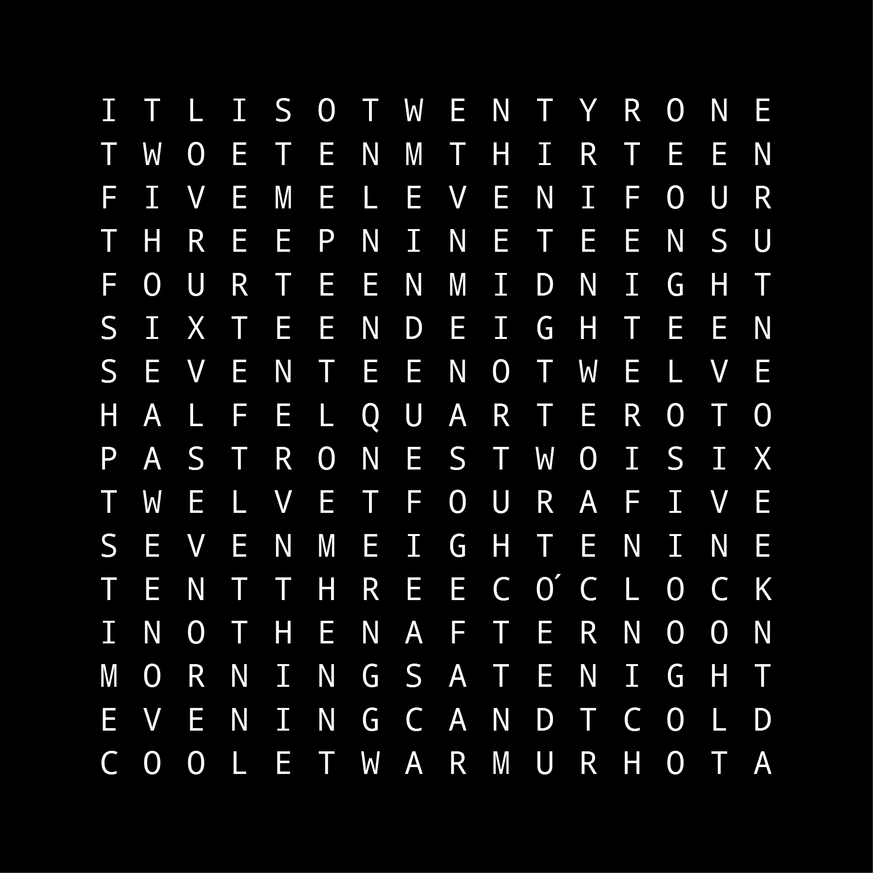
"One across, nine letters: C-blank-O-blank-S-blank-blank-R-blank" *

I've always assumed that running this on the client-side in JavaScript would be far too slow. It turns out I was very wrong; if you're careful with your coding, you can get it running in a browser on a low-end tablet or phone with memory and CPU cycles to spare.

My first problem was getting hold of a good lexicon or word list. The obvious avenue to explore was the "official" Scrabble word list used in competitions, but it quickly became apparent that there are at least two such lists:

• The Official Tournament and Club Word List (or, more specifically, "TWL06" for the 2006 version) used in USA, Canada and Thailand ; and
• SOWPODS used just about everywhere else.

These are simply lists of words that are considered "valid"; the former is over 178,000 words and the latter over 267,000 words. They do not contain definitions nor any metadata about the words such as frequency.

In contrast, SCOWL (Spell Checker Oriented Word Lists) contains over 423,000 words with information such as relative frequency and regional variations (American/Canadian/British). Some of the words are suspect (domain-specific abbreviations and bad optical character recognition are two likely sources of suspicious "words") but the frequency information makes it easy to cull outliers.

Instead of choosing just one word list, I decided to go for all three and divided the superset of words into five levels of "rarity" based on the SCOWL frequency metadata. It turns out that SOWPODS is a superset of TWL06, but contains some words not found in SCOWL.

After a lot of curation (in Excel, of all tools!) I ended up with a list of 432,852 words split into five levels of increasing "rarity". Each word is implicitly tagged with the word lists in which it is found. I limited the words to those between two and fifteen letters (inclusive) where each "letter" is one of the twenty-six Roman letters "A" to "Z" (no digits, apostrophes, hyphens or accents are allowed).

I could have stored the lexicon as a simple text file or as a JSON array of strings, but this would have taken up several megabytes, so I decided to have a go at trivial compression. I know, I know ... most HTTP servers will serve up compressed files out of the box and there exist any number of JavaScript libraries that do client-side decompression of ZIP files, but I felt like re-inventing a wheel. Give me a break!

The main constraint I gave myself was to try to get the lexicon to the client-side in a usable form as quickly as possible. This meant a trade-off between file size and time taken to decompress and store in a suitable data structure. One thing you don't want to do is sort half a million words into alphabetical order on the client. That means the lexicon (or parts thereof) needs to be pre-sorted.

Sorted word lists have a lot of redundancy at the beginning of each entry. For example, imagine a list starting like this:

• AARDVARK
• AARDVARKS
• AARDWOLF
• AARDWOLVES
• ...

If we replace the beginning of each word with a digit ('0' to '9') specifying how many letters from the previous word we should replicate, the list becomes:

• 0AARDVARK
• 8S
• 4WOLF
• 7VES
• ...

Another technique is to substitute common letter sequences with ASCII characters outside the ranges '0' to '9' and 'A' to 'Z'. It turns out that the most common four-letter sequences near the end of the words are:

NESS TION ABLE ICAL MENT INGS LESS

For three-letter sequences, the list is:

ING OUS IES ATE TIC TER ISM IST SES INE ION IVE 

While the most common near-end two-letter sequences are:

ED ER ES AL LY AN IC EN IT OR IS ON AR LE IN IA ST ID RA PH UL LA OM IL CH TE CE US UR AT OL

Using these two simple techniques, the 432,852 words can be compressed into a single ASCII string of just over 1.5 million characters. This string can be efficiently converted into a high-performance in-memory data structure within a second on a typical PC.

The full demo can be found here, whilst the JavaScript file that decompresses the word list is lexicond.js.

* "CLOISTERS" obviously

Modulo Arithmetic and Days of the Week

Yesterday, I noticed something curious about the Wikipedia entries for days of the year. Here's an example from January 1:

The text that caught my eye is:

This date is slightly more likely to fall on a Tuesday, Friday or Sunday (58 in 400 years each) than on Wednesday or Thursday (57), and slightly less likely to occur on a Monday or Saturday (56).

Huh? At first I thought this was an obvious mistake; surely the days of the week are evenly distributed. After all, there are 365 or 366 days in a year and 7 days in a week, and these numbers are relatively prime.

Here's my (erroneous) line of reasoning:

1. Neither 365 nor 366 are divisible by 7. [True]
2. Therefore, January 1 can be any day of the week. [True]
3. The "leap year" cycle repeats after 400 years. [True]
4. But 400 is not divisible by 7. [True]
5. Therefore, the "leap year and January 1 weekday" cycle repeats every 2800 years. [False]

My mistake was trying to divide 7 (the number of weekdays) into 400 (the number of years in a "leap year" cycle). What I should have done is try to divide 7 into the number of days in a "leap year" cycle.

So, how many days are there in 400 full years? Well, there are (100 - 4 + 1) = 97 leap days, so there are (365 * 400 + 97) = 146097 days.

Amazingly, 146097 is divisible by 7, so the "leap year and January 1 weekday" cycle repeats every 400 years, not every 2800 years. As we know, 400 is not divisible by 7, so this cycle cannot possibly have a uniform distribution of weekdays for January 1.

Indeed, even leap days (February 29) are not immune from this lack of uniformity because 97 is not divisible by 7. In any 400 year period, there are:

• Thirteen each of Mondays, Wednesdays and Fridays,
• Fourteen each of Saturdays and Sundays, and
• Fifteen each of Tuesdays and Thursdays.

At this point in the discussion, someone usually witters on about calendar reform.

So why not...

Imagine reforming the calendar such that January 1 is always a Saturday but without forsaking the 7-day weekly cycle. One scheme would be to have a 52-week standard year (364 days) with periodic "leap weeks" (371 days). If we define a leap year to be any year that is divisible by 6 or 62 we end up with a 186-year leap cycle with 153 standard years and 33 leap years, making a total of (153 * 364 + 33 * 371) = 67935 days. That implies that the mean year length is (67935 / 186) = 365.2419355 which is closer to the solar year of roughly 365.242181 days than the current Gregorian calendar (365.2425).

So here's the new scheme:

• A standard year is 364 days, divided into 52 weeks of seven days.
• A month is defined as 4 weeks or 28 days. There are thirteen months in a year.
• A leap year consists of 371 days with the extra "special" week of festivities tacked on to the end.
• A year is a leap year if it is divisible by 6 or 62.
• All years, months and weeks begin on Saturday.

Strange, but this seems vaguely familiar...

Lost in Translation T-Shirt

Lost in Translation

Blok Clok

When I was a boy, I was given a curious present: a perpetual desk calendar made from wooden cubes:

You can still buy them, so there must be some enduring appeal. The calendar interested me because of a strange quirk that isn't immediately obvious.

There are four blocks: one for the day of the week (with seven labels), two for the day of the month (1 to 31) and one for the month (with twelve labels). The "weekday" and "month" blocks are easy to label. For example, two months on each face fills the "month" block and, providing the container covers up the lower half of the block, all is peachy.

The two date blocks are a little more involved. Dates run from "01" to "31":

01,02,03,04,05,06,07,08,09,10,  

11,12,13,14,15,16,17,18,19,20,  

21,22,23,24,25,26,27,28,29,30,31

By inspection, we see that the only digits that appear twice on a single date are "1" and "2". However, if you sit down with a pencil and paper, it quickly becomes apparent that you'll also need two zeroes. That means that the following digits are required:

0,0,1,1,2,2,3,4,5,6,7,8,9

But, hang on! That's thirteen digits. Two cubes have only twelve faces between them. How do they fit? The clever "quirk" is that "6" and "9" occupy the same face; you simply flip the block around 180 degrees. This gives you the following faces for the two blocks:

0,1,2,3,4,5

0,1,2,6,7,8

This arrangement allows to you represent all integers between "00" to "32" inclusive; just enough! It's deceptively clever. And that's probably why I like my wooden perpetual calendar so much.

Fast forward several years, if not decades, and my current fascination with clocks led me to consider whether you could tell the time with a similar arrangement. I knew representing the hours would not be a problem: as we've seen, two blocks can represent all integers between "00" to "23" inclusive for a twenty-four-hour clock. But representing minutes is harder.

It is fairly obvious that you need at least three blocks to represent all integers between "00" to "59" inclusive. But are three sufficient? It turns out that they are; you don't even need to use the upside-down "9" trick. The solution uses an additional cube to display a colon between the hours and minutes digits. For example:

23:59

The "tens minutes" digit takes up a single block: "0" to "5" inclusive. So the problem simplifies to trying to represent the "units minutes" digit ("0" to "9") and a colon with two blocks. The following labelling is one solution:

:,0,1,2,3,4

:,5,6,7,8,9

Using three blocks to represent minutes between ":00" to ":59" inclusive can be repeated for the seconds. This gives us eight blocks:

  hours-a    0,1,2,3,4,5

  hours-b    0,1,2,6,7,8

minutes-a    :,0,1,2,3,4

minutes-b    0,1,2,3,4,5

minutes-c    :,5,6,7,8,9

seconds-a    :,0,1,2,3,4

seconds-b    0,1,2,3,4,5

seconds-c    :,5,6,7,8,9

Not only do the blocks need to rotate to any of their six faces (and in the case of "hours-b", the "6" sometimes has to be flipped to become a "9") but pairs of blocks also have to be swapped periodically:

hours-a <=> hours-b

minutes-a <=> minutes-c

seconds-a <=> seconds-c

Some extra fettling is needed to make the rotations aesthetically pleasing, but the result is a twenty-four-hour clock that twists and turns at a fair old lick.

Minimal Rotor Clock

The Rotor Clock I posted about last month is all very well, but there are a heck of a lot of moving parts: thirty-two rotors, each with ten faces. You could physically build it, but things would be a lot easier if there were fewer components. So I set about trying to reduce the number of rotors for a twelve-hour clock that displays the time as words.

The extreme (degenerate) case is a single rotor with 12 * 60 = 1440 faces. This would produce a working clock, but the rotor would need to be enormous (or the text very small). The next idea I had was a clock with two rotors: one for hours and one for minutes. You could repeat the twelve hours five times and make both rotors have 60 faces. This would still require very large rotors. Also, telling the time in a "natural" British English manner is quite tricky. Consider:

QUARTER TO TWELVE

TWELVE O'CLOCK

FOURTEEN MINUTES PAST TWELVE

The solution I came up with (which may not be optimal, but is possibly close) is to use four rotors, each with at most twelve words or phrases plus a blank face:

    Rotor A      Rotor B      Rotor C         Rotor D
    =======      =======      =======         =======
    THIRTEEN     ONE          O'CLOCK         ONE
    FOURTEEN     TWO          MINUTE PAST     TWO
    SIXTEEN      THREE        MINUTES PAST    THREE
    SEVENTEEN    FOUR         QUARTER PAST    FOUR
    EIGHTEEN     FIVE         HALF PAST       FIVE
    NINETEEN     SIX          QUARTER TO      SIX
    TWENTY       SEVEN        MINUTES TO      SEVEN
                 EIGHT        MINUTE TO       EIGHT
                 NINE                         NINE
                 TEN                          TEN
                 ELEVEN                       ELEVEN
                 TWELVE                       TWELVE

Note that rotor B is identical to rotor D.

This produces a clock that can tell the time as hoped for, but with the insertion of another blank face in rotor A and a bit of duplication in rotor C, I was able to reduce the number of large rotations quite considerably. This produces a series of relatively smooth transitions. The final rotors are organised thus:

    Rotor A      Rotor B      Rotor C         Rotor D
    =======      =======      =======         =======
    (blank)      (blank)      (blank)         (blank)
    THIRTEEN     ONE          O'CLOCK         ONE
    FOURTEEN     TWO          MINUTE PAST     TWO
    (blank)      THREE        MINUTES PAST    THREE
    SIXTEEN      FOUR         QUARTER PAST    FOUR
    SEVENTEEN    FIVE         MINUTES PAST    FIVE
    EIGHTEEN     SIX          HALF PAST       SIX
    NINETEEN     SEVEN        MINUTES TO      SEVEN
    TWENTY       EIGHT        QUARTER TO      EIGHT
    (blank)      NINE         MINUTES TO      NINE
    (blank)      TEN          MINUTE TO       TEN
    (blank)      ELEVEN       (blank)         ELEVEN
    (blank)      TWELVE       (blank)         TWELVE

If you look at the JavaScript code, you'll see that control of the rotors is via two data tables. This scheme lends itself to efficient compression. Indeed, a slightly cut-down variation of the clock can be compressed into a single 1017-byte HTML page (providing you're using a highly-compliant browser such as Google Chrome or Mozilla Firefox).

Word Time 1KB

One of my inspirations for the Rotor Clock was the Instructables wordclock that tells the time (and temperature) based on a 16-by-16 grid of letters:

It looked very much like a puzzle to me, so I immediately set about trying to work out the minimum size of grid that could tell the time to an accuracy of one minute. I managed to get the grid down to 13-by-13:

TWENTYQUARTER

TWONETHIRTEEN

FOURTEENTHREE

SEVENTEENFIVE

TWELVEIGHTEEN

IDTENSIXTEENT

ELEVENINETEEN

MINUTESHALFTO

PASTBFOURNOON

MIDNIGHTWONED

THREELEVENSIX

FIVEIGHTENINE

SEVENZO'CLOCK

[I have a suspicion you can get it even smaller if you use tricks such as spelling words vertically; but, after a considerable amount of effort, I plumped for 13-by-13]

In my usual modus operandi, I then tried to optimise the heck out of the problem by hand and attempt to fit a solution into a one-kilobyte web page that works on Chrome, Firefox and Internet Explorer. For added frisson, I didn't allow myself to use non-ASCII characters nor the evil JavaScript "eval()" or its ilk. The result, World Time, takes up just 1023 bytes:

Here's a quick breakdown of the contents:

We can omit a large number HTML elements such as "DOCTYPE", "head" and "body" and dive straight into the style definitions, which are assumed by browsers to be CSS. We set all backgrounds to black, centre the table in the middle of the page and format each table cell so that a 13-by-13 grid takes up most of the viewport. The default text colour is set to very dark grey and a shadow effect is added to simulate "light bleed":

We then define a table that will hold the 169 grid characters and be accessed in the JavaScript via a identifier named "t". The string is split into 169 table cells (each one 10 characters of HTML) which are then divided into 13 rows:

Next we decode a 78-character string that has been btoa-encoded (so we adhere to our ASCII restriction). The 78 characters represent 39 pairs of offsets into the "t" grid. The first of each pair is the "start" offset (0 to 168); the second is the "end" offset plus one. These 39 pairs define tokens with even numbers identifying them thus:

           #00 = "O'CLOCK"
           #02 = "MINUTE"
           #04 = "MINUTES"
           #06 = "PAST"
           #08 = "TO"
           #10 = "HALF"
    #12 to #38 = "ONE" to "FOURTEEN" (upper portion)
           #40 = "QUARTER"
    #42 to #50 = "SIXTEEN" to "TWENTY"
           #52 = "MIDNIGHT"
    #54 to #74 = "ONE" to "ELEVEN" (lower portion)
           #76 = "NOON"

These 38 tokens constitute all the words used by the clock. See below for details of the call to "setInterval":

Next, we define a function "d()" that takes two arguments (the third argument declaration is just a short way of declaring a variable - see 140bytes for other such techniques), The first argument is the hour as an integer. The second argument is either "00" (the token for "O'CLOCK") or "" depending on requirements. The "d()" function therefore returns the hour as a string of two-digit tokens (e.g. "7400" for "ELEVEN O'CLOCK"). It has a special case for "MIDNIGHT" and "NOON" which never take the "O'CLOCK" suffix:

We define another function "g()" that takes an integer number of minutes (0 to 59) as its only argument. It returns a string of tokens representing the appropriate number of minutes as words (e.g. "(something) MINUTES" or "TWENTY (something) MINUTES", taking into consideration the exceptional cases for "ONE MINUTE", "QUARTER" and "HALF". Note that we're playing fast and loose with the type system here: the number 1202 will be converted to the string "1202" elsewhere in the program.

Next, we define an anonymous function (let's call it "storeColours") that takes one true argument ("b" is a local variable declaration again). This is called with the result of another anonymous function ("calculateColours") that takes three arguments: the current local hour, the current local minute and an empty dictionary. The "calculateColours" function constructs a full string of tokens that describe the current time. If the minute value is zero, we use the "d()" function to construct "MIDNIGHT", "NOON" or "(hour) O'CLOCK". If the minute value is less than or equal to thirty, it constructs "(something) PAST (hour)". Otherwise, if constructs "(something) TO (hour+1)". The string of tokens are split into two-digit numbers and looked up in the "s" table described above. For every letter in every word, "calculateColours" stores an HSL colour in the "c" dictionary keyed by the appropriate offset into the grid. The dictionary is then passed to "storeColours" which modifies the style text colour of each table cell in turn. Setting the colour to "" results in the text colour reverting to the colour defined in the CSS entry for "td" (i.e. very dark grey):

Finally, we invoke the "calculateColours" and "storeColours" function at most every 1000 milliseconds via the "setInterval" function mentioned above, and gracefully close the HTML tags.

A lot of the JavaScript compression came from Google Closure Compiler.

The result is a colourful clock that spells out the time in English words, uses a responsive HTML layout and takes the local timezone, changes in daylight savings and even leap-seconds into consideration.

UPDATE: 2016-06-29

I've managed to shave an additional ten bytes off the size and updated the page, but the structure and technique are essentially the same as above.

Rotor Clock

There seems to be a bit of fad for clocks that spell out the time. There are even some online examples utilising a variety of languages. And jolly good they are too!

Spelling out the time in British English is fairly simple. Just take the local time and extract the minutes. If the value is less than thirty, express the time as

  (minutes) PAST (hour)

Otherwise, use

  (60-minutes) TO (hour+1)

There are some exceptional cases; if the minute value is zero, use

  (hour) O'CLOCK

Whereas minute values or 15, 30 and 45 are generally expressed as

  QUARTER PAST (hour)
  HALF PAST (hour)

  QUARTER TO (hour+1)

It turns out that, using the above scheme, the maximum number of characters needed to spell out the time is 32. For example:

  TWENTY SEVEN MINUTES PAST TWELVE

If we are a little bit lenient with the spacing between the words, we can prune the number of distinct characters in each position to ten (including space). This leads to an interesting configuration for a mechanical device that can spell out the time using 32 rotors of only 10 facets each.

With a little bit of CSS3 and HTML5, it's possible to produce a web page that brings such a device to life. If you further optimise the HTML, CSS and Javascript, you can present it in a single file of only 2191 bytes.

A Short History of Long Ships

With the recent maiden voyage of "MS Harmony of the Seas," there's been a lot of talk in the press about large and long ships. So here's my attempt at a summary:

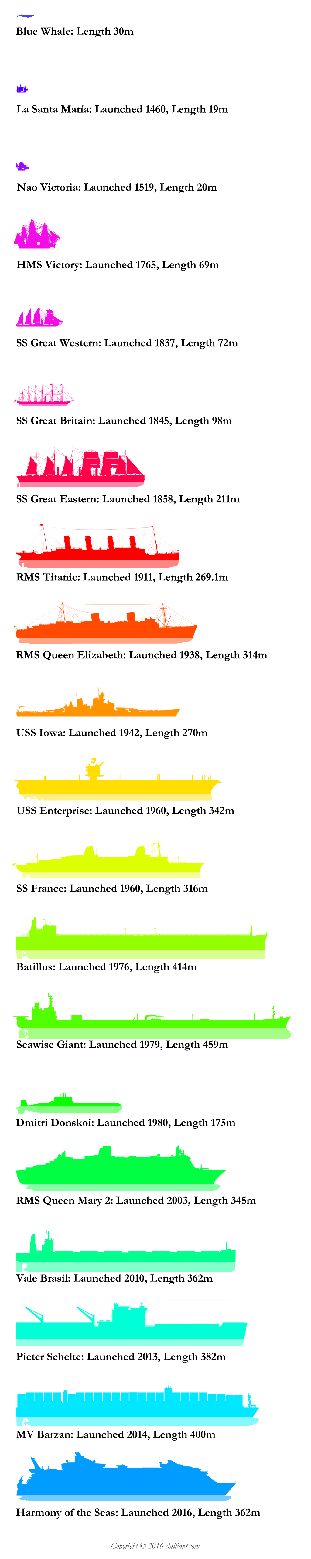
The blue whale is the largest extant animal.

La Santa María, launched in 1460, was largest of three ships used by Christopher Columbus to cross the Atlantic for the first time in 1492. She ran aground later in 1492.

The Nao Victoria, launched in 1519, was the first ship to circumnavigate the globe in 1522. She disappeared in 1570.

HMS Victory, launched in 1765, was Nelson's flagship at the Battle of Trafalgar in 1805. She is still in service.

SS Great Western, launched in 1837, was the largest passenger ship until 1839. She was broken up in 1856.

SS Great Britain, launched in 1843, was the longest passenger ship until 1854. She was finally scuttled in the Falklands in 1937.

SS Great Eastern, launched in 1858, was the longest ship built of any type until 1899. She was scrapped in 1889.

RMS Titanic, launched in 1911, was the largest ship afloat until she sunk on her maiden voyage in 1912.

RMS Queen Elizabeth, launched in 1938, was the largest (by displacement) passenger liner for almost fifty years. She finally caught fire and sunk in Hong Kong harbour in 1975.

USS Iowa, launched in 1942 and now a museum ship, is the longest battleship ever built. The Japanese Yamato was more massive, but slightly shorter.

The aircraft carrier USS Enterprise, launched in 1960, is the longest naval vessel ever built. She was decommissioned in 2012, but, being nuclear powered, she will take a long time to be completely dismantled.

SS France, launched in 1960, took over from RMS Queen Elizabeth as being the longest passenger ship. She was sold for scrap in 2005.

Batillus, launched in 1976, was the largest supertanker by gross tonnage ever built. She was scrapped in 1976.

Seawise Giant, launched in 1979, was the longest ship ever built. She was scrapped in 2010.

Dmitri Donskoi, launched in 1980, is a Typhoon-class submarine, the largest in the world. She is still in active service.

RMS Queen Mary 2, launched in 2003, is the largest ocean liner ever built. She is still in service.

Vale Brasil, launched in 2010, is the largest bulk carrier ever built. She is still in service.

Pieter Schelte, launched in 2013, is the largest vessel ever constructed in terms of gross tonnage, breadth and displacement. She is still in service.

MV Barzan, launched in 2014, is the largest container ship ever built. She is still in service.

MS Harmony of the Seas, launched in 2015, is the largest passenger ship in the world by gross tonnage. She entered service in May 2016.

The maximum length of ships in service is usually limited by canal sizes and port facilities.

See here for a larger image.

JavaScript Flags 3

As mentioned in the previous post, the JavaScript Flags hobby project encodes the drawing instructions for each flag as a string. For examples, the Japanese flag is encoded as

"FwCrO+0+0+72"

This is split up into a sequence of instructions or commands using a regular expression match:

[ 
  ["F", "w"], 
  ["C", "r"], 
  ["O", "+0", "+0", "+72"] 
]

The first element of each instruction is always a single upper-case letter. The remaining elements are either lower-case letters usually indicating colours (see the previous post) or signed integers (expressed as strings). Often, the integers represent coordinates. No matter what the aspect ratio of the flag, the top-left corner is always (-120,-120) and the bottom-right is (+120,+120). Two hundred and forty was chosen because it fits into a byte (although that's not important for this JavaScript implementation of the flag renderer) and is highly divisible.

The command letters are as follows:

• "A n" — Executes the next command in the sequence "n" times, rotating about the origin by (360 ÷ "n") degrees each time.
• "B x y path ..." — Draws a path made up of a mixture of straight-line and cubic Bezier segments and fills it with the current colour. See below.
• "C c" — Sets the current colour to "c",
• "D f w" — Draws diagonal lines of width "w". If "f" is 1, a diagonal line from top-left to bottom-right is drawn. If "f" is 2, a diagonal line from top-right to bottom-left is drawn. And if "f" is 3, both diagonals are drawn.
• "E sx sy" — Executes the next command with scaling about the origin. If either "sx" or "sy" are negative, executes the next command twice: once with scaling (abs(sx),abs(sy)) and once with scaling (sx,sy). Otherwise, just executes the next command with scaling (sx,sy).
• "F c" — Fills the entire canvas with solid colour "c".
• "H c y0 y1" — Draws a full-width, horizontal block in colour "c" between y0 and y1, where y0 < y1.
• "J" — Draws a union flag in the top-left quadrant.
• "M x y path ..." — Draws a mirrored path made up of a mixture of straight-line and cubic Bezier segments and fills it with the current colour. See below.
• "O cx cy r" — Draws and fills with the current colour a circle of radius "r" centred at (cx,cy).
• "P n c[0] ..." — Draws "n" horizontal stripes. The colour of stripe "i" (where 0 ≤ i < n) is "c[i % m]" where "m" is the number of colour arguments, c.
• "Q n c[0] ..." — Draws "n" vertical stripes. The colour of stripe "i" (where 0 ≤ i < n) is "c[i % m]" where "m" is the number of colour arguments, c.
• "R x0 y0 x1 y1" — Draws and fills an axis-aligned rectangle with the current colour between (x0,y0) and (x1,y1).
• "S x y r" or "S n r1 r2 x y a" — With three arguments, draws a five-pointed star filled with the current colour at (x,y) and radius "r". With six arguments, draws an "n"-pointed star filled with the current colour at (x,y), inner radius "r1" and outer radius "r2" all rotated by "a" degrees.
• "T x0 y1 x1 y0" — Draws and fills a right-angled, axis-aligned triangle whose hypotenuse is (x0,y0) to (x1,y1).
• "V c y0 y1" — Draws a full-height, vertical block in colour "c" between x0 and x1, where x0 < x1.
• "X c w x" — Draws an axis-aligned cross of width "w" in colour "c". The vertical bar passed through the x-axis at "x", The horizontal bar is along the x-axis.
• "Y n dx dy" — Executes the next command in the sequence "n" times, translating by (dx,dy) after each iteration.
• "Z x0 y0 x1 y1" — Zooms in to a rectangle (x0,y0) and (x1,y1) where x0 < x1 and y0 < y1. All subsequent commands assume the 240-by-240 canvas is now (x0,y0) to (x1,y1).

The paths for the "B" and "M" commands start and finish at (x,y). The intervening points are prefixed by a lower-case letter:

• "l x y" — Lower-case "L" — A straight-line segment  from the previous point to (x,y).
• "s x1 y1 x y" — Lower-case "S" — A smooth cubic Bezier segment from the previous point to (x,y) with control point (x1,y1).
• "c x1 y1 x2 y2 x y" — Lower-case "C" — A general cubic Bezier segment from the previous point to (x,y) with control points (x1,y1) and  (x2,y2).

For the "M" command, the path is mirrored about a vertical axis centred on the final point of the explicitly-specified path. This allows emblems such as the double-headed Albanian eagle to be encoded very efficiently.

In summary, less than twenty commands encode the instructions for drawing most of the world's flags very effectively. The use of regular expression string splitting and function lookup maps in JavaScript makes the encoded strings short whilst keeping the decoding code equally concise,

JavaScript Flags 2

As promised, I thought I'd take time to document some of the code behind my JavaScript flags hobby project. If you look at the data file for the flags, flagdata.js, you'll see a single JSONP-style JavaScript call:

Flags({
  AD:["Andorra",10/7,"..."],
  ...
  BL:["Saint-Barthelemy","FR"],
  ...
  JP:["Japan",3/2,"FwCrO+0+0+72"],
  ...
  ZW:["Zimbabwe",2,"..."]
});

The single argument is an object with ISO-3166 two-letter codes as keys and arrays of two or three elements as values. If the array has three elements, they are:

1. The country or territory name, as a string;
2. The flag's aspect ratio, as a rational floating-point number; and
3. The instructions for drawing the flag, as a string (see below).

If the array has only two elements, they are:

1. The country or territory name, as a string;
2. The ISO-3166 code of the "parent" country whose flag this entry shares, as a two letter string.

The latter scheme allows "aliases" to be set up for flags that are shared by more than one territory:

• France
• Netherlands
• Norway
• United States of America

The instructions for drawing the flags as represented as a string. The pseudo-BNF of these instructions is as follows:

instructions ::= instruction ... 
instruction ::= command argument … 
command ::= 'A'..'Z' 
argument ::= number | colour 
number ::= sign digit ... 
sign ::= '+' | '-' 
digit ::= '0'..'9' 
colour ::= 'a'..'z'

It is therefore trivial to parse these instruction streams using regular expressions. For example, Japan has the following entry:

JP:["Japan",3/2,"FwCrO+0+0+72"]

The instruction stream can be split into individual instructions using:

instructions.match(/([A-Z][^A-Z]*)/g)

This produces an array:

["Fw", "Cr", "O+0+0+72"]

These three instructions can be further divided into numbers (which are always preceded with a sign) and single-letter colours:

instruction.match(/.\d*/g)

This produces an array for each instruction:

[
  ["F", "w"],
  ["C", "r"],
  ["O", "+0", "+0", "+72"]
]

The first element is thus always an upper-case letter and is used as the key into a map for commands. I'll discuss the meaning of each letter (command) next time. Subsequent elements in the instruction array are arguments to the command: numbers and/or colours. Colours are always lower-case letters:

a: #39F light-blue
b: #00F medium-blue
c: #009 dark-blue
g: #CCC grey
m: #630 brown
n: #000 black
o: #F60 dark-orange
p: #F90 light-orange
r: #F00 bright-red
s: #C00 medium-red
t: #900 dark-red
u: #060 dark-green
v: #090 medium-green
w: #FFF white
y: #FF0 yellow

But for now, we'll finish off the Japanese flag example by expanding the instruction arrays:

fill white
colour bright-red
circle +0 +0 +72

This would get translated by the JavaScript code in flags.js to the following pseudo-SVG:

svg viewbox="0 0 360 240" xmlns="http://www.w3.org/2000/svg"
  g stroke="none" transform="matrix(1.5,0,0,-1,180,120)"
    g
      rect fill="#FFF" height="240" width="240" x="-120" y="-120" /
      ellipse cx="+0" cy="+0" fill="#F00" rx="48" ry="+72" /
    /g
  /g
/svg